Download Microsoft.77-427.PracticeTest.2018-11-11.4q.tqb

Vendor:	Microsoft
Exam Code:	77-427
Exam Name:	Excel 2013 Expert Part One
Date:	Nov 11, 2018
File Size:	2 MB

Download Exam

Demo Questions

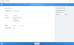
Conditional Formatting.

Use a formula to determine formatting of a cell.

Cell I3

Apply formatting if cell is more than three days prior to current date

Use Function TODAY()

Format with Custom solid fill color (RGB – R:255 G:59 B:59)

Use the following steps in explanation.

Correct answer: A

Explanation:

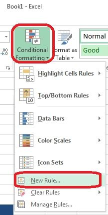
Step 1: Click cell I3.Step 2: In the Home tab, click Conditional Formatting, and select New Rule. Step 3: In the New Formatting Rule dialog box select Use a formula to determine which cells to format, in the Formal Values where this formula is true type: =TODAY()-I3>3, and then click the Format button. Step 4: In the Format Cells dialog box click the Fill tab, click More Colors, in the Colors Dialog box click the Custom tab, change Green to 59, change Blue to 59, click OK, click OK, and finally click OK in the New Formatting Rule dialog box.

Step 1: Click cell I3.

Step 2: In the Home tab, click Conditional Formatting, and select New Rule.

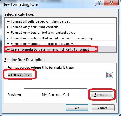
Step 3: In the New Formatting Rule dialog box select Use a formula to determine which cells to format, in the Formal Values where this formula is true type: =TODAY()-I3>3, and then click the Format button.

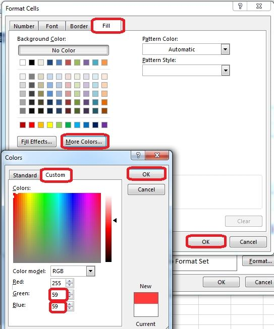
Step 4: In the Format Cells dialog box click the Fill tab, click More Colors, in the Colors Dialog box click the Custom tab, change Green to 59, change Blue to 59, click OK, click OK, and finally click OK in the New Formatting Rule dialog box.

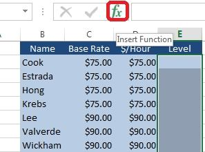
Use a function to insert a value in a cell.

Cell range E2:E44

The "Level" of each employee

Function LOOKUP (vector form)

Lookup_value: "$/Hour" (Column D)

Lookup_Vector: Lower Limit row from table.

Use the following steps in explanation.

Correct answer: A

Explanation:

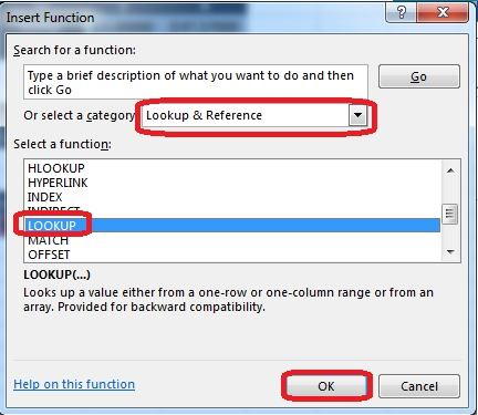
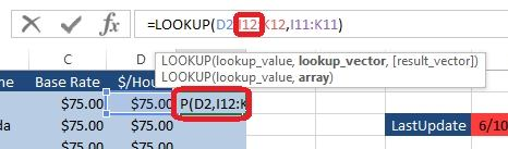
Step 1: Click cell E2, and click the Insert Function button. Step 2: In the Insert Function dialog box select Category Lookup & Reference, select function LOOKUP, and click the OK button. Step 3: In the Select Arguments dialog box make sure lookup, value, lookup vector, result vector is select and click OK. Step 4: For Lookup_value click cell D2, for Lookup_vector select cells I12:K12, for Result vector cells I11:K11, and click the OK button. Step 5: Click cell E2, click in cell reference I12 in the formula field, and press the F4 key (to make I12 an absolute reference. Step 6: Make K12, I11 and K11 absolute references using F4 in the same way.Result will be: Step 7: Click cell E2, and copy downwards to E44. Result will be like:

Step 1: Click cell E2, and click the Insert Function button.

Step 2: In the Insert Function dialog box select Category Lookup & Reference, select function LOOKUP, and click the OK button.

Step 3: In the Select Arguments dialog box make sure lookup, value, lookup vector, result vector is select and click OK.

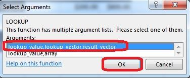
Step 4: For Lookup_value click cell D2, for Lookup_vector select cells I12:K12, for Result vector cells I11:K11, and click the OK button.

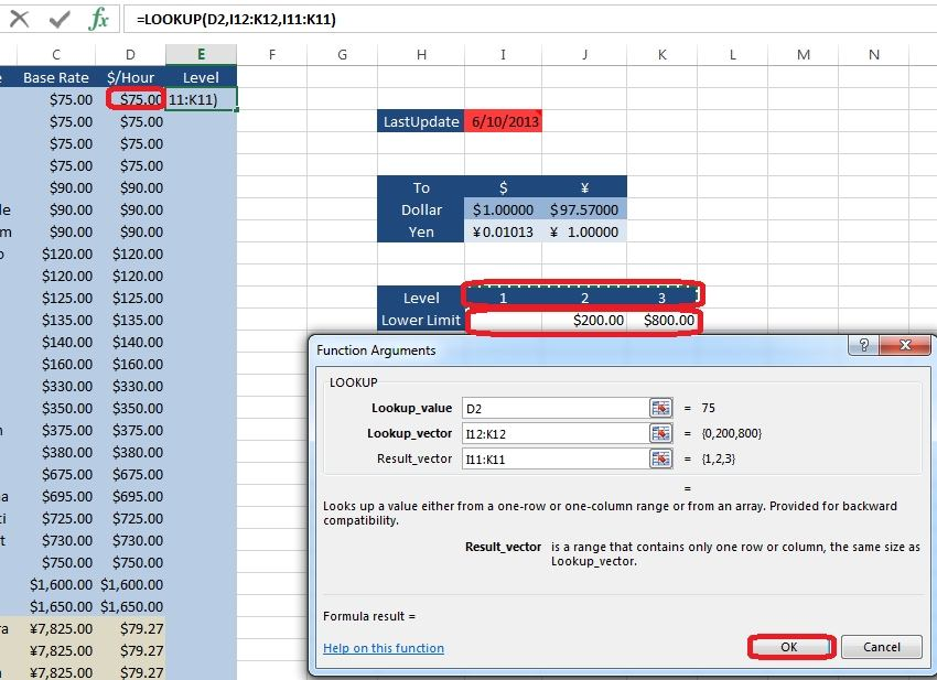
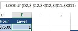
Step 5: Click cell E2, click in cell reference I12 in the formula field, and press the F4 key (to make I12 an absolute reference.

Step 6: Make K12, I11 and K11 absolute references using F4 in the same way.

Result will be:

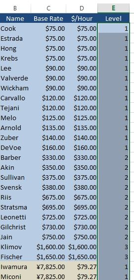
Step 7: Click cell E2, and copy downwards to E44.

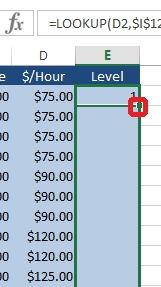
Result will be like:

Apply conditional formatting using a formula.

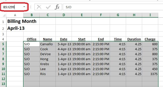
Cell range B5:I299

Apply if "Date" (column D) is a Saturday or Sunday

Function WEEKDAY (return MONDAY as 0)

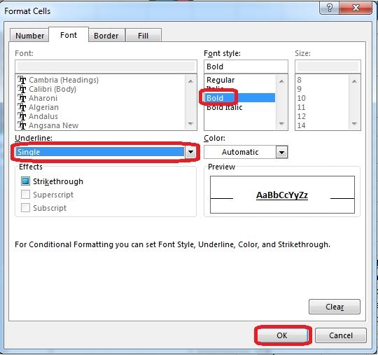
Formatting Bold and Single Underline

Use the following steps in explanation.

Correct answer: A

Explanation:

Step 1: In the name box type B5:I299 (or Click cell B5, shift-click cell I299). Step 2: On the Home tab, select Conditional Formatting, and click New Rule Step 3: In The Edit Formatting Rule dialog box select Use a formula to determine which cells to format, type the formula: =WEEKDAY($D5,2)>5, and click the Format button. Step 4: In the Format Cells dialog box select bold, Underline Single, and click OK. Step 5: In The Edit Formatting Rule dialog box click Ok.

Step 1: In the name box type B5:I299 (or Click cell B5, shift-click cell I299).

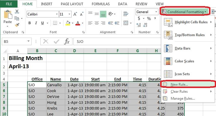
Step 2: On the Home tab, select Conditional Formatting, and click New Rule

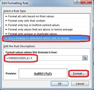
Step 3: In The Edit Formatting Rule dialog box select Use a formula to determine which cells to format, type the formula: =WEEKDAY($D5,2)>5, and click the Format button.